
“Serial killer” is a term customarily used to refer to a person who has murdered three or more people over a period of more than a month. Perhaps the most infamous of these criminals is Jack the Ripper, who terrorised the streets of London in the year 1888.
The Ripper’s Whitechapel Murders included, the United Kingdom has a rich and disturbing history of serial killers – from the Body Snatchers (William Burke and William Hare, 1828), through Brides in the Bath (George Smith, 1912–1914), to the murders at 10 Rillington Place (John Christie, 1943–1953) and the Grindr Killer (Stephen Port, 2014–2015).
The rarity, cruelty, and debauchery of serial killers has the power to fascinate and repulse us. Their vicious murders fuel newspaper articles, true-crime bestsellers and blockbuster movies. But they may also inspire others to commit similar heinous acts.
A copycat crime is one that is modelled on a previous crime – thus a copycat killer is someone inspired by another murderer. The “copycat effect” is said to have been coined around 1916 as a result of Jack the Ripper’s crimes being mimicked; it refers to the imitation of crimes as a result of the publicity attributed to the originals. The Ripper is believed to have been the muse for a number of killers. However, he is seemingly not the only figure from whom killers draw their inspiration.
Dr Thomas Neill Cream, the Lambeth Poisoner, qualified as a surgeon in Edinburgh in 1878. Between 1877 and 1892, in both Chicago and London, he is said to have poisoned nine people, including five prostitutes: Mary Faulkner, 1880; Ellen Donworth and Matilda Clover, 1891; and Alice Marsh and Emma Shrivell, 1892. On 15 November 1892 Dr Cream was hanged at Newgate prison. Whilst on the scaffold with the noose around his neck, some claim he yelled, “I am Jack”, thus inferring that he was Jack the Ripper. This is, in fact, impossible: at the time of Jack’s crimes, Dr Cream was serving a prison sentence for poisoning his mistress’s husband, Mr Daniel Stott, in 1881.
In 2008 Derek Brown was convicted of murdering an illegal Chinese immigrant, Xiao Mei Guo, and a prostitute, Bonnie Barrett. Their bodies have never been found, but Brown’s flat contained equipment that may have aided in their disposal. Allegedly, Brown was driven to kill by a wish to emulate Jack the Ripper; he reportedly had numerous books on the subject.
Mark Rowntree tormented the county in the mid-1970s – at the same time as the Yorkshire Ripper, Peter Sutcliffe, began his series of murders (13 in total) in the North of England. Despite being classified as a serial killer, many would consider Rowntree a spree killer as his four victims were all killed in one week. He is said to have claimed that his only regret was not killing as many people as The Black Panther, Donald Nielson. The Black Panther was convicted, among other crimes, of murdering four people in Yorkshire and the Midlands between 1974-1975.
The urges that serial killers seek to gratify are no doubt unfathomable to the majority of us. However, there may be some motivating processes that may be inferred through the application of statistical analysis. In what follows, I attempt to discern a pattern in the crimes of Britain’s serial killers by considering the dates of their first murder as statistical occurrences.
TABLE 1 Number of recorded serial killers in Britain from 1828 to 2014, along with the approximate number of murders they committed. In some cases the number of murders reported is an estimate (e.g., Dr Harold Shipman was suspected of 300+ murders but only convicted of 15).
| Years | Number of serial killers | Approximate number of murders | Notorious killers |
| 1828-1859 | 4 | 38 | William Burke & William Hare (Body Snatchers) |
| 1860-1890 | 3 | 35 | Jack the Ripper |
| 1891-1921 | 3 | 9 | George Chapman (The Borough Poisoner) |
| 1922-1952 | 6 | 193 | John Christie (10 Rillington Place), and John George Haigh (Acid Bath Murderer) |
| 1953-1983 | 22 | 171 | Ian Brady & Myra Hindley, Fred & Rosemary West, and Peter Sutcliffe (The Yorkshire Ripper) |
| 1984-2014 | 24 | 385 | Dr Harold Shipman and Stephen Port (The Grindr Killer) |
A copycat (self-exciting) process
Trends over time may be best thought of as rates: the number of red herrings per Agatha Christie mystery, or the number of times Sherlock Holmes berates Watson in a story. It is simple to evaluate this heuristically, and the steps are as follows: first, take a sub-sample of books; second, sum the number of occurrences; third, divide by the number of novels. This gives a single number, a constant rate of occurrence. But what if things don’t occur at a constant rate? What if there is an underlying process that changes over time? What if the rate is partially dependant on its history?
Temporal intensity describes the rate of occurrence of some event over time. If this intensity changes over time it is typically denoted λ(t), meaning that it is a function of time. That is, it is not simply a constant rate but includes some additional term that describes the form of temporal dependence. This extension to the constant rate may be thought of as consisting of two components: one, the underlying baseline rate; two, a term describing the jump in rate after an event has occurred. The latter term may be formulated so that it describes behaviour similar to that of a copycat. That is, every time an event occurs the rate of the process jumps upwards, expecting further copycat events to follow. If a period of time elapses without any events then the rate steadily declines – copycat events are most likely to occur soon after the events they imitate. Such an intensity process is not simply dependent on time, but assumes additional dependence on historical events. This intensity is, in fact, that of a Hawkes process1 with the following mathematical formulation:


This is called the branching ratio of the process, and gives the average number of events that occur as a result of a preceding event.
Given these two ways of describing the rate of occurrences, can we tell if the occurrence of a serial killer at any one time is equally likely? That is, do they come around at random? In an attempt to answer this question, we consider the two aforementioned processes: one that says serial killers occur randomly in time, the other that says serial killers may be more likely to come about if a previous killer strikes (i.e., a self-exciting process).
How many serial killers does it take to…
To infer if there is some pattern evident in the murders committed by British serial killers, let us assume that the first kill date is a statistical event (i.e., each event relates to one killer). Table 1 shows the number of recorded unique serial killers from 1828 until 2014, as well as the approximate number of murders in that period; notorious killers of the associated time periods are also named. These data were obtained from the MurderUK website.2 It should be noted that in some cases only the date pertaining to the first murder of which the perpetrator was convicted is used, despite the perpetrator being suspected of many other murders. In addition, in some cases the number of murders is an estimate (e.g., Dr Harold Shipman was believed to have committed far more murders than those for which he was convicted). From Table 1, it might seem that the number of serial killers is quite dissimilar in each period, which gives rise to some questions: Is the number of serial killers growing? Is the rate of murders by serial killers increasing?
Let us initially assume that the rate of these events is constant over time, and that there is no dependence on historical events. There are 62 recorded events (serial killers) in 186 years, giving an average of 0.3 (recurring) events per year; this constant rate is represented by the horizontal dashed line in Figure 1. Next, let us consider a Hawkes process to explain the rate of the first barbarous deeds of serial killers – this assumes that the temporal intensity has some self-excitement (copycat) property. Using this model, we obtain the estimates of μ = 0.078, α = 0.06, and β = 0.065; these estimates give raise to the solid grey line in Figure 1. So, according to this model, there is a base rate of 0.078 serial killers per year, with each killer seemingly inspiring more.
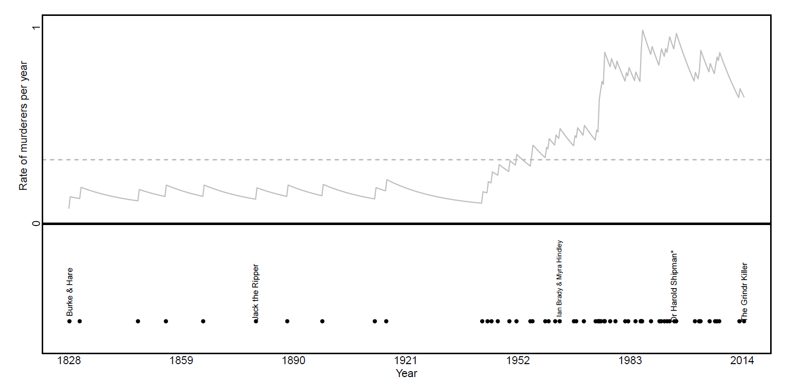
FIGURE 1 Fitted intensities for both the copycat process (solid grey line), and a process with constant rate (dashed horizontal line). Each event relates to the date of the first murder committed by each serial killer. The bottom panel indicates these dates from the year 1828 until 2014. Some notorious serial killers are included. The horizontal dashed line is the fitted flat line intensity to all events, the solid grey line is the self-exciting intensity. *Note that in the case of Dr Harold Shipman, as in some other cases, only the first murder for which he was convicted is used, although he was suspected of many more prior to this.
Clearly there are more murderers by serial killers evident from around 1950 onwards (see Table 1). One rather obvious reason for this increase is the growth in Britain’s population, which was about 16 million in 1828 and is approximately 65 million now. Therefore, in order to more correctly talk about the rate of serial killers, we should account for this population growth. This is achieved by essentially scaling the Hawkes rate shown in Figure 1; the result of this scaling is shown in Figure 2. The copycat formulation of the intensity is still preserved; however, now the rate is given as number of serial killers per year per million people. This rate seems to be at its maximum in the 1980s with an estimate of approximately 0.016 serial killers per year per million, and at its lowest around the 1940s with around 0.002 serial killers per million. As expected, the difference in rate of killers pre- and post-1950 is dampened when we account for population density, but Figure 2 still shows an increase in more recent decades.
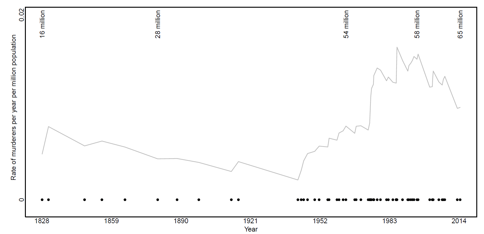
FIGURE 2 The fitted copycat intensity, where now the rate is given as the number of serial killers per year per million people. Estimated population of the UK (in millions) is indicated for certain years.
As noted above, there are evidently more serial killers from around 1950 onwards, and the self-exciting intensity seemingly reflects this better than the rather inflexible constant intensity. We can use a common piece of statistical machinery – a likelihood-ratio test – to see if the extra complication in the Hawkes process is necessary. Having turned the handle on this particular statistical machine, we find that the model accounting for copycat murderers is unsurprisingly and overwhelmingly preferred to using the restrictive constant intensity.
Few of us will be able to, or will want to, understand the perverse mental drivers of serial killers. Yet statistics offers us the chance to perhaps ascertain some pattern in their atrocities. Assuming that a Hawkes process describes the behaviour of serial killers enabled us to account for copycat behaviour; we assume some dependence on historical events (i.e., other killers) rather than simply dependence on time. There are of course numerous other effects that are likely to contribute to the ever-changing rate of serial killers, not least the efficiency and effectiveness of our police force. If murderers are caught before they have the chance to kill again, our estimated intensity is sure to decline. But even then, our morbid fascination with serial killers seems unlikely to diminish.
About the author
Charlotte Moragh Jones-Todd graduated with a PhD in statistics from the University of St Andrews in June of this year. Her PhD focused mainly on the modelling of spatial and spatio-temporal point pattern data. She is currently living in Auckland, New Zealand working as a postdoctoral research consultant.
Charlotte’s article was a runner-up in the 2017 Statistical Excellence Award for Early-Career Writing. The winning article, by Kevin Lin, is published here. Details of next year’s competition will be announced in February 2018.
References
- Alan G Hawkes and David Oakes. A cluster process representation of a self-exciting process. Journal of Applied Probability, 11(03):493–503, 1974. ^
- Terry Hayden. MurderUK: documenting and investigating murder in the UK. URL http://www.murderuk.com/serial_killers/html. Accessed: 01-05-2017. ^


