
Social distancing is important in controlling the spread of Covid-19. This strategy has proven to be highly effective in flattening the curve of new cases/deaths. In this article I discuss the spatial implications of England’s social distancing policy in relation to the school setting and, in particular, how this might apply to seating configurations in schools as the Covid-19 lockdown, implemented from 23 March 2020, is gradually eased.
The following discussion would also be relevant to spatial considerations for the design of open-plan offices and the placement of office workers’ desks.
Social distancing and the concept of “zones of influence”
The social distancing policy in England recommends that individuals maintain a spatial distance of “1 metre plus”, but that people should stay 2 metres apart where possible to minimise the spread of the virus. The concept of social distancing can be illustrated using the concept of zones of influence: suppose that each individual has a zone of influence around them, and when two individuals have overlapping zones of influence, transmission of the virus can occur.
For a social distancing policy with 2 metres as the specified distance, we can consider each zone of influence to have a radius equal to 1 metre, since this would imply no interaction when individuals are more than two metres apart and gradually increasing interaction as their separation is reduced below two metres. A radius of 1 metre does not have a direct interpretation; in particular, it does not imply that an individual can only spread the virus 1 metre in any direction.
The zone of influence1,2 can be thought of as the region within which an individual is able to exert an impact on another in a spatial context. This concept has traditionally been used in modelling the spatial locations of plants/animals: the zone of influence in the case of plants, for example, could reflect the impact an individual plant can have on the soil nutrients available to another neighbouring plant.
In this application, the value of the radius can also be considered to be a function of variables such as the density of the area (city centre, park, etc.) and the concentration of the virus particles.
Of course, immediate challenges would then be to determine:
- whether some individuals would have a larger zone of influence/infection than others;
- whether the “true” zone of influence has a radius of 1 metre;
- how long the virus can persist on air pollution particles;
- the spatial distribution of large cough particles relative to smaller ones; and
- the difference in the concentration of cough particles at the back/front of an infected person (reinforcing the idea that the radius r may not be fixed but be a function, in this case, of the direction the person is facing).
Researchers (Yulia Parshina-Kottas et al. and Knvul Sheikh et al.) have indicated that the particles in a cough may travel further than 6 feet (which is approximately 2 metres); especially the smaller particles. In particular, they note that larger particles are quicker to fall to the ground while smaller particles can remain in the air and persist for a relatively longer period of time.
Illustration of zones of influence in the presence of a simulated cough cloud
Using the concept of zones of influence and the variation of particle size in a given cough cloud, Figure 1 represents a simulated point pattern containing the location of 13 students (black dots) in the presence of a cough cloud. The darker yellow regions denote the area of overlap between each student’s zone of influence (discs around each point) with that of their nearest neighbours. The radius of each circle (zone of influence) is 1 metre; as a result any overlap between the zones of influence would by greater than zero only if the students are at least 2 metres apart.

Figure 1: Fifteen individuals randomly distributed within an enclosed square of 10 x 10 metres.
The red dots represent larger and heavier infected airborne water droplets within a cough cloud from the student (who we’ll call “Psi”) with Covid-19; the green dots represent smaller particles in that cough cloud which form an aerosol. In this illustration, I have simulated the cough particles so that the particles represented in red and green fall within the zone of influence of Psi. The purple dots represent small cough particles that travel further than the radius of the zone of influence, under the assumption that the true radius of the zone of influence is greater than 1 metre. If the true zone of influence has a radius greater than 1 metre, the students would need to be distanced from each other at a distance greater than 2 metres. This ensures that their zones of influence do not overlap.
A hypothetical classroom of 25 split into two
Let us consider a hypothetical class of 25 students, originally in one classroom. After national advice to reduce class size, this class is now split into two, such that there are two resulting classes, each in separate rooms. For a given school with n classes undergoing such a transformation, there is a need to ensure that 2 × n rooms are available. Possibly, if necessary, the classes can be kept in the same original classroom, but the groups of students attend classes at different shifts – morning and afternoon.
The aim for the following simulations is to illustrate the change in the area of non-overlap of the zones of influence associated with different spatial arrangements of students within an enclosed room. The size of the classroom is arbitrary.
A cluster of 15 students
Let us consider one subset (15 students) of the abovementioned class of 25 students, such that this group of students attends class in a separate room and the students from this subset interact only with other students from this subset.
If these students maintain social distancing of 2 metres, the area of non-overlap between their zones of influence is most likely to be less than if they were instead spatially random. Note that for the simulation of spatially random points, I have used a Poisson point process model. Technical details on simulating point patterns can be found here.
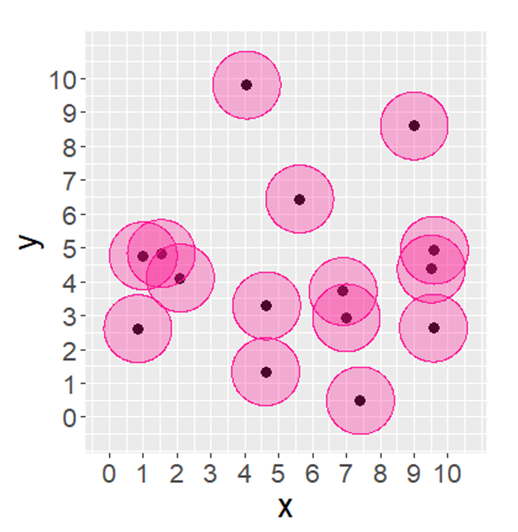
Figure 2: Fifteen students randomly distributed within an enclosed square of 10 × 10 metres.
In Figure 2, the points represent 15 students who are randomly distributed within an enclosed room of 10 x 10 metres. Note that this represents just one instantiation of a random spatial pattern.
The area of non-overlap of their zones of influence is 31.8m2 and the percentage of non-overlap is 67.4%. If there was complete social distancing of 2 metres, the area of non-overlap of the zones of influence would be 47.1 m2 as shown in Figure 3, with 100% non-overlap.
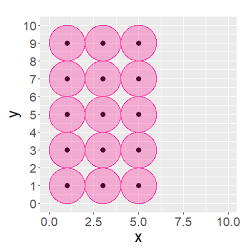
Figure 3: Fifteen students distributed in a regular spatial configuration within an enclosed square of 10 × 10 metres. Each student is 2 metres away from each other.
In contrast, Figure 4 illustrates the same 15 students now regularly spaced just 1 metre apart. In this example, the area of non-overlap of the zones of influence is 7.3 m2. This represents 15.4% of the total area of the zones of influence.

Figure 4: Fifteen students distributed in a regular spatial configuration within an enclosed square of 10 x 10 metres. Each student is 1 metre away from each other.
So, why should we examine what the spatial implications of social distancing would mean in classrooms?
- Adherence to social distancing within schools will require spatial adjustments to the normal layout of the school environment.
- A reduction in classroom size to, at most, 15 will necessitate the provision of additional classrooms for the remainder of students within a given class who do not fall within this cluster.
- Assessing the level of social distancing would be facilitated by the concept of area of non-overlap of zones of influence.
About the author
Dr Glenna Nightingale is a research fellow (statistician) in the Scottish Collaboration for Public Health Research and Policy, School of Health in Social Science, The University of Edinburgh.
References
- Nightingale, G. F., Illian, J. B., King, R., and Nightingale, P. (2019) Area Interaction Point Processes for Bivariate Point Patterns in a Bayesian Context. Journal of Environmental Statistics, 9(2), 1-21. ^
- Picard, N., Bar-Hen, A., Mortier, F., and Chadœuf, J. (2009) The Multi-scale Marked Area-interaction Point Processes: A Model for the Spatial Pattern of Trees. Scandinavian Journal of Statistics, 36(1), 23-41. ^


