How many people are infected now with the novel coronavirus, SARS-CoV-2? How many will be infected tomorrow? These are hard questions because we can’t just see who is infected, and we don’t know how each infected person is interacting with others, either infecting them or not. Here I’ll explain the basic framework used to estimate how many people are likely to become sick, and how many will recover or die. There’s some notation, but I’ll present each equation in words. At this level, we’re reasoning more with logic than with math.
Why isn’t this just arithmetic?
In the United States, there is a severe shortage of tests for SARS-CoV-2, the virus that causes people to become sick with the disease known as Covid-19. As a consequence, even people in the hospital with obvious and severe symptoms of Covid-19 are rarely tested for the virus. Furthermore, it is by now becoming clearer that many, perhaps most people infected with SARS-CoV-2 have mild or no symptoms. The combination of these factors means that only a small fraction of the SARS-CoV-2 cases are ever confirmed by a positive test. In practice, the confirmed case counts tell us more about the availability and distribution of tests than the prevalence of infections. Consequently, the true number of SARS-CoV-2 positive individuals is necessarily much higher than the reported counts. But how much higher?
The total size of the infected population determines how many people will need critical care, and how many will ultimately die. It is therefore important for healthcare planning, economic policy, and public communication to estimate the population prevalence of SARS-CoV-2 infection.
The foundation of epidemiological modeling is the SIR model. This model enables us to estimate the progression, day by day, of the sizes of three sub-populations: those who are Susceptible, Infectious, and Removed.
On each day, some of those who are susceptible get infected, and themselves become infectious to other people. The number of people who become infected is a combination of how contagious the disease is, as well as the effectiveness of social distancing, handwashing, and other practices that can limit transmission.
Similarly, on each day, some of those who are infected will recover or die, and these people are no longer at risk of transmitting the disease. We call these people “removed”, in the sense that they are “removed” from the infected population.
This model is dynamic which means that it changes over time. To understand what’s happening today, each component of the model depends on what was happening yesterday with the other components.
The notation and meaning
Scientists often convert word problems into notation that lets us see connections among the pieces and then do calculations. Here’s how the pieces of the SIR model fit together.
On any given day, the population can be divided into the people still susceptible to the virus, the people infected with the virus, and the people who have been “removed”, that is, either recovered or died. We’ll write this as N = St + It + Rt , where the subscript t means “this day”. Naturally that means that the subscript t – 1 means “the day before this day”. Keep in mind that the R term includes both people no longer sick and those who have died.
Deaths
We can observe the number of deaths on each day:
Dt
This is pretty much the only part of the pandemic we can measure without a lot of uncertainty. (There’s still a little error because not all deaths due to Covid-19 are reported correctly, and some deaths that aren’t due to Covid-19 might be reported in error.)
Susceptible (S)
“Susceptible” in this context means “available to become infected”. The number of people (in a population N ) who are susceptible on day t equals the number susceptible yesterday minus the people who are newly infected today (νt ):
St = St – 1 – νt
Note that as long as people can only be infected once, the number of susceptible people can only go down.
Recovered
This isn’t usually defined as a separate term, but it’s worth noticing that the number of people who recover and are no longer sick each day is some fraction (γ ) of all the people infected through yesterday, minus all the people who died through yesterday:
γ (It –1 – Dt –1)
The γ term is a proportion between zero and one, and it tells us how many people are recovering. Most SIR models lump together the “recovered + dead”, but I think it’s useful to think about them as separate processes. I’ll use this definition of “recovered” in the next two definitions.
Infected (I)
The number of infected people on day t equals the number infected yesterday, plus the people newly infected today, minus the people who died yesterday, minus the people who recovered yesterday (note the recovered term at the end):
It = It –1 + νt – Dt –1 – γ (It –1 – Dt –1)
This number can go up as new infections occur and down as people recover and die.
Removed (R)
The number of people removed on day t equals the number removed yesterday, plus the people who died yesterday, plus the people who recovered yesterday (note the recovered term at the end):
Rt = Rt –1 + Dt –1 + γ (It –1 – Dt –1)
Note that as long as people can only be infected once, the number of removed people can only go up.
Newly infected
The number of new infections each day is equal to the number of susceptible people yesterday times some fraction (β ) of the infected proportion. The infected proportion is simply the proportion of the population who was infected yesterday:
The β term is a measure of infectiousness. β is mathematically related to the epidemiological term R0 , which is the average number of people that each infected person newly infects. I’ve shown it here as β rather than R0 so that the role of “infectiousness” can be clear in the math relating the susceptible and infected populations.
Infected fatality rate
The fraction of the infected people who will eventually die equals the total deaths (summing all the daily totals) divided by the total people ever infected:
This rate may change as healthcare is overloaded, or as new treatments are discovered. It is different for people of different ages and different “co-morbidities” like diabetes, hypertension, and smoking. There is still considerable debate about the p number for Covid-19, which is usually expressed as a percent. Most sources report that p seems to be between 0.5–2.0%, averaged across various studies, various age groups, and various co-morbidities.
Putting it all together
We can estimate the SIR values by using the relationships among them and information from clinical studies. The New York Times has an interactive online tool which allows a user to see immediately the effect of changing any of these parameters. Covid-19 can be understood as a generic epidemic which has its own values of these parameters. Of course, policy and human behavior influence the parameters too, by reducing transmission through social distancing, reducing fatalities through better treatment, and ultimately, reducing susceptibility through a vaccine. The processes over time can be seen in Figure 1.
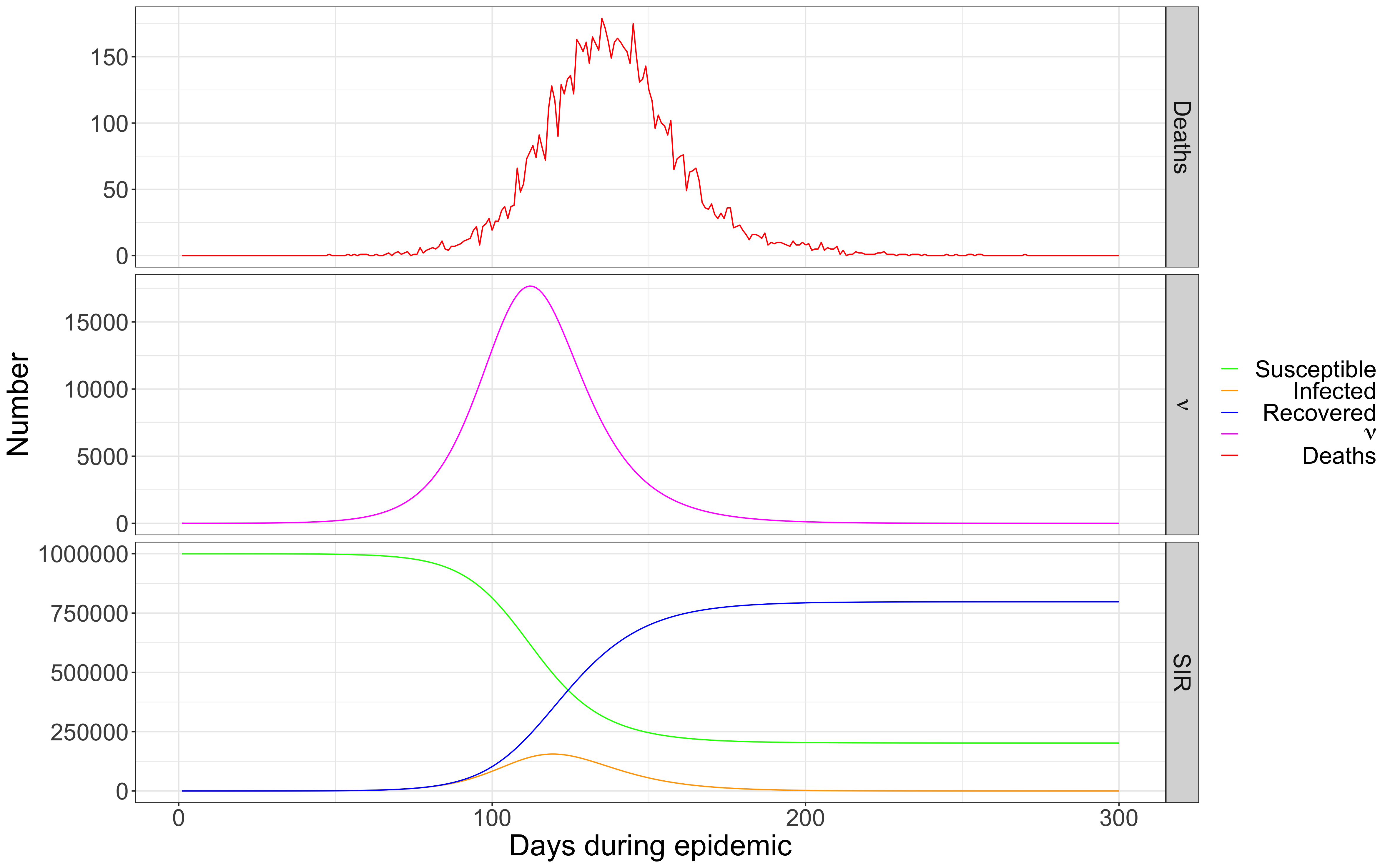
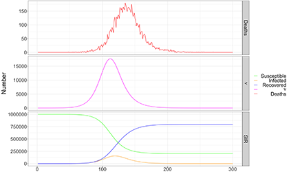
FIGURE 1 Deaths, susceptible, infected, and removed in a hypothetical population (from Johndrow et al.).
The top graph shows the number of deaths each day, which is the only measure we can really observe. The middle graph shows the number of new infections each day. Note that it leads the deaths by a couple of weeks, and the length of this lead is another variable in the model which can only be observed through limited clinical studies. The bottom graph shows the SIR values: the susceptible population (the green line) starts with everyone and declines over time. The infected group rises for a while then slowly declines. The removed population rises over time, eventually including everyone—the dead and the survivors.
Different modeling projects approach this framework differently. Which parts are assumed, measured, or modeled vary among different studies. Some models let the interactive user guess different values of R0 (and thereby β ) or p (and thereby γ ), while other models incorporate measures from small clinical studies. Some models include an intervening term, exposure, between the susceptible population and infection (not all susceptible people are exposed, and the unexposed people cannot become infected). The math that connects all the pieces is also different in different models.
In the long term, we’ll learn which models were best. However, time is too short for more than a tiny number of these models to be subject to formal peer review in time to be relevant. That means it is more important than ever that engaged laypeople (especially journalists) have at least a minimum sense of how to read these essential studies.
Further reading on the SIR model
Kermack W., and A. McKendrick (1927) “A contribution to the mathematical theory of epidemics.” Proceedings of the Royal Society of London Series A: Mathematical and Physical Sciences 115: 700-721.
Anderson RM and RM May (1991) Infectious Diseases of Humans. Oxford Science Publications, Great Britain.
Acknowledgements
I’m interpreting these ideas from a paper by James Johndrow, Kristian Lum, and me (the preprint is on arXiv). I am grateful for their comments, as well as for suggestions from Maria Gargiulo, Megan Price, Tarak Shah, Stella Pierce, Danielle Fugere, Hope Howard, and Jacob Nelson.
About the author
Patrick Ball is director of research at the Human Rights Data Analysis Group.


