
Spatial data make an enormous contribution to our understanding of the world. They allow us to monitor life expectancy and the spread of disease within a country, the distribution of employment and wealth across a continent, and the condition and use of land in a conservation area. They help us to understand from where people watched the recent eclipse, which roads are the most dangerous, and what areas of a city are the least polluted and have the lowest crime rates.
Recently, an enormous effort has been put into producing tools for visualising spatial data and it is easy to find a vast number of examples. However, these mainly concentrate on colouring geographical regions according to the average value of a variable to produce a choropleth type map, or adding a scatter plot of (x,y) data to an area.1-4 Sometimes, more sophisticated visualisations are associated with geographical regions, but these may be time-consuming or require a dedicated team to produce.
The ggplot22 package is a plotting system for R, based on the book The Grammar of Graphics.5 It is now the graphics tool of choice for many people, including journalists, because it allows a wide range of graphs to be produced and fine-tuned in a reproducible way. One of its key features is “faceting”, which automates the generation of similar plots for subsets of the data. Recently, Ryan Hafen contributed an R package called geofacet that “provides geofaceting functionality for ggplot2” and which “arranges a sequence of plots of data for different geographical entities into a grid that strives to preserve some of the original geographical orientation of the entities”.6 Hafen illustrates the use of his package for the states of the USA, the countries of the EU and several other geographical regions by producing bar plots and time series visualisations. In principle, it is easy to create grids for different countries and regions, and users are encouraged to submit these through github.
The aim of this short article is to provide a further illustration of the use of the geofacet package by displaying population data from the 20 regions of Italy using a grid that we have produced. We believe that Hafen’s geofacet package makes a powerful, but simple-to-use contribution to visualising spatial data, and we hope that this contribution will encourage the production of grids for other geographical regions.
Italy has 20 regions and these are shown in Figure 1. The shape of the country and the positioning of its districts make the construction of a suitable facet grid difficult.
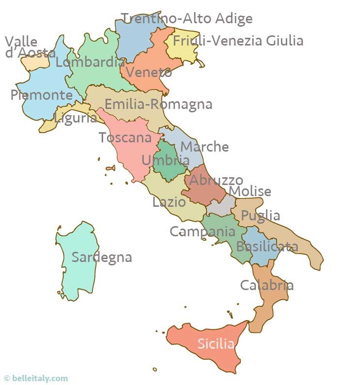
FIGURE 1 The 20 regions of Italy (source).
All the population data that we now present were extracted from the Italian National Institute of Statistics, ISTAT. Figure 2 shows the population of the 20 regions from 1992 to 2017. We can see from Figure 2 that there is a vast difference in population sizes between regions. Lombardy (LOM), for example, is a highly populated region, while Valle d’Aosta (VAL) is a sparsely inhabited, small, mountainous area. Figure 2 allows us to see the main difference in the population sizes of the Italian regions, but much of the detail of the variation is lost because the same scale is used for each facet. Nevertheless, population increases are visible for some regions, such as the northern Lombardy (LOM), Veneto (VEN) and Emilia-Romagna (EMI) cluster.
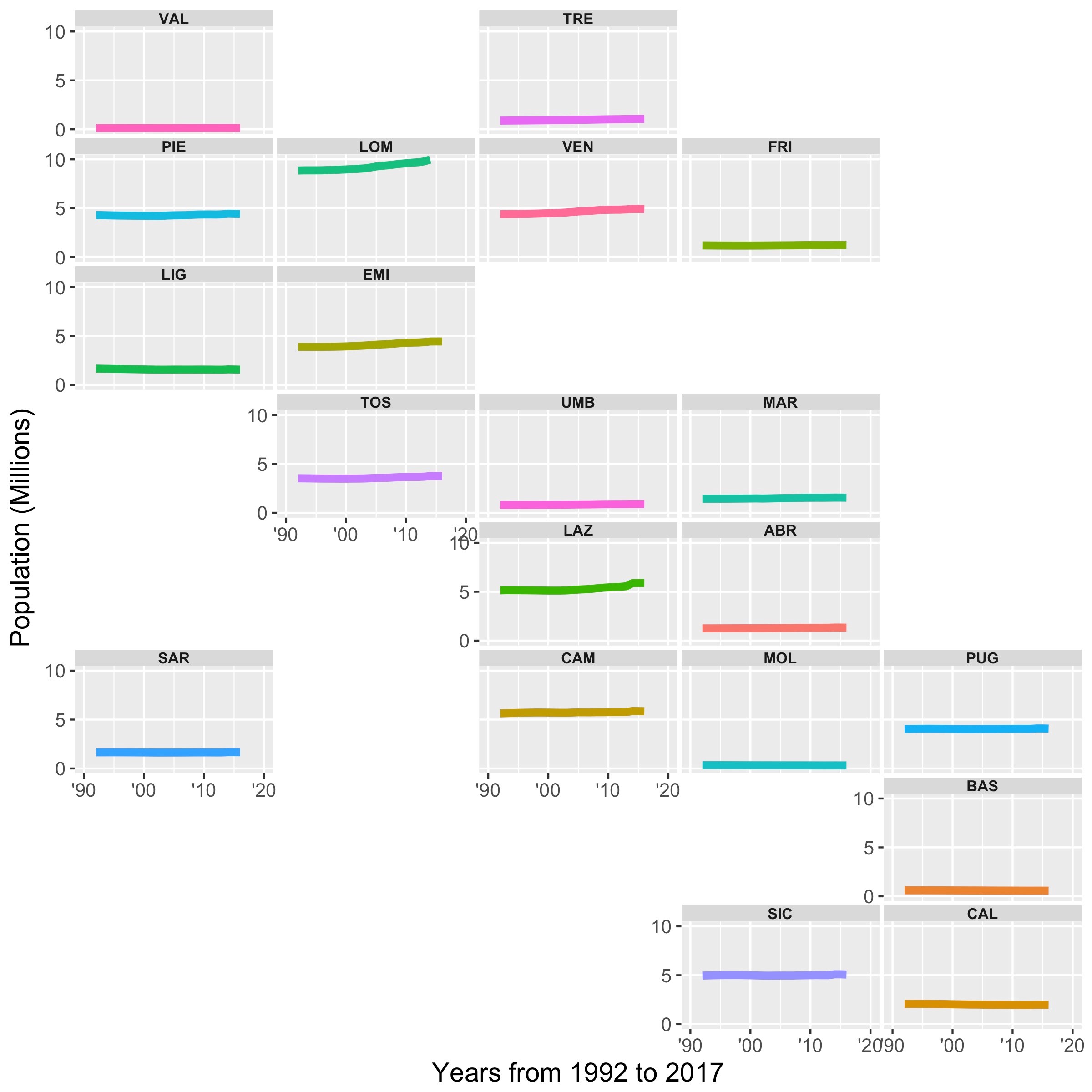
FIGURE 2 The population of the 20 Italian regions from 1992 to 2017. Standard abbreviations are used for the region names.
Figure 3 shows the percentage population increase for the 20 regions using 1992 as the baseline. This simple data transformation allows the variation within each region to be seen more clearly as now population increases – rather than levels – are shown. We observe that there is a cluster of southern regions, comprising Molise (MOL), Basilicata (BAS) and Calabria (CAL), where the population has been declining. The percentage population increases for the island regions of Sicily (SIC) and Sardinia (SAR) are essentially zero, while northern regions including Trentino-Alto Adige (TRE), Lombardia (LOM), Veneto (VEN) and Emilia-Romagna (EMI) have seen strong population growth.
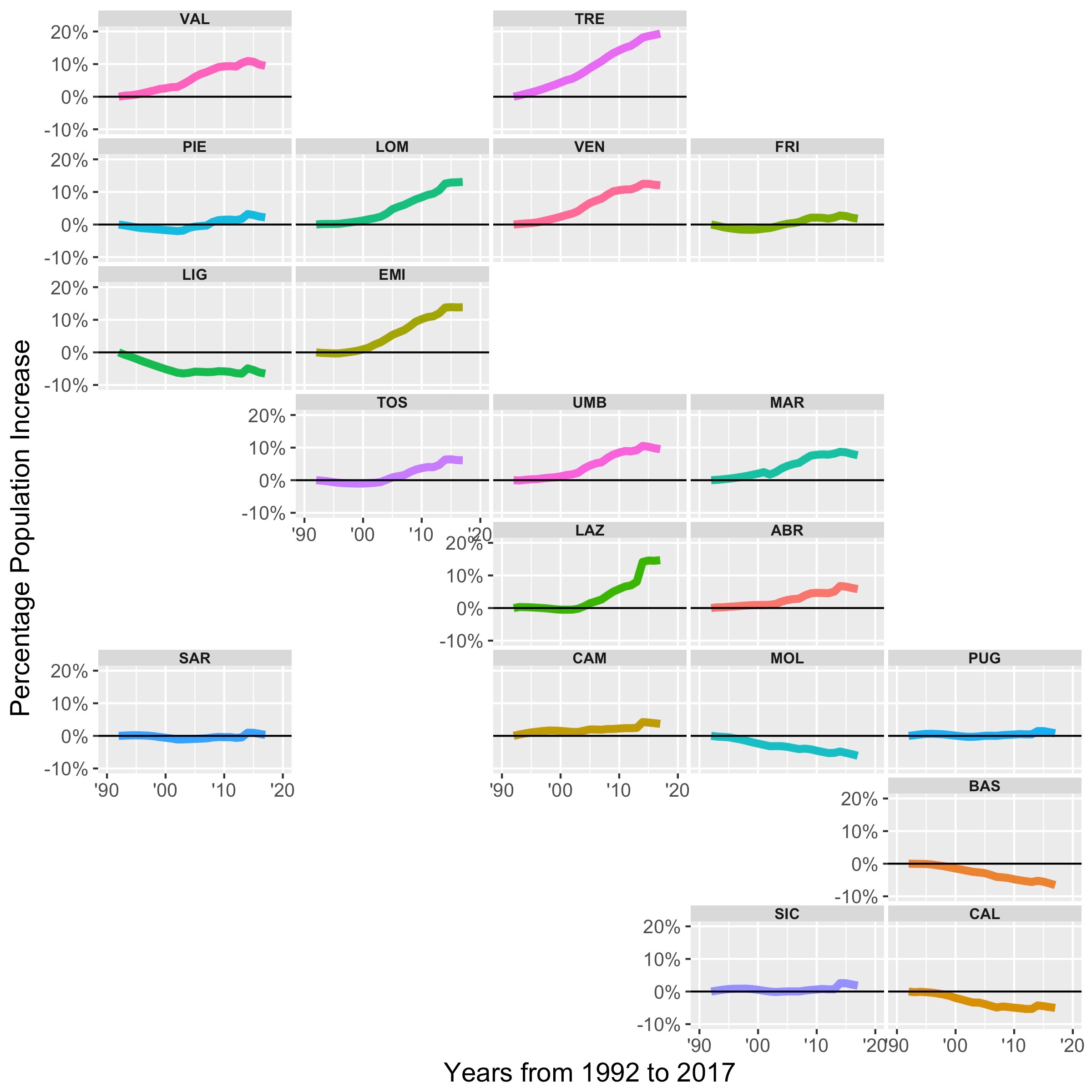
FIGURE 3 The percentage population of the 20 Italian regions from 1992 to 2017.
Finally, Figure 4 shows the percentage of people in the population who are over 75 years (in red) or under 5 years (in blue). We see that in every region the percentage of people over 75 years has increased over time. The decline in the percentage of children under 5 years in some of the southern regions – Campania (CAM), Molise (MOL), Puglia (PUG), Basilicata (BAS) and Calabria (CAL) – and the islands of Sicily (SIC) and Sardinia (SAR) is evident. The reasons for this decline and the fact that Italy has one of the lowest birth rates in the world are complicated. They may be related to a reduction in economic prosperity and thus the employment prospects of younger people, together with the changing effects on fertility of women’s employment, with noticeable differences being present between northern and southern regions.7-10
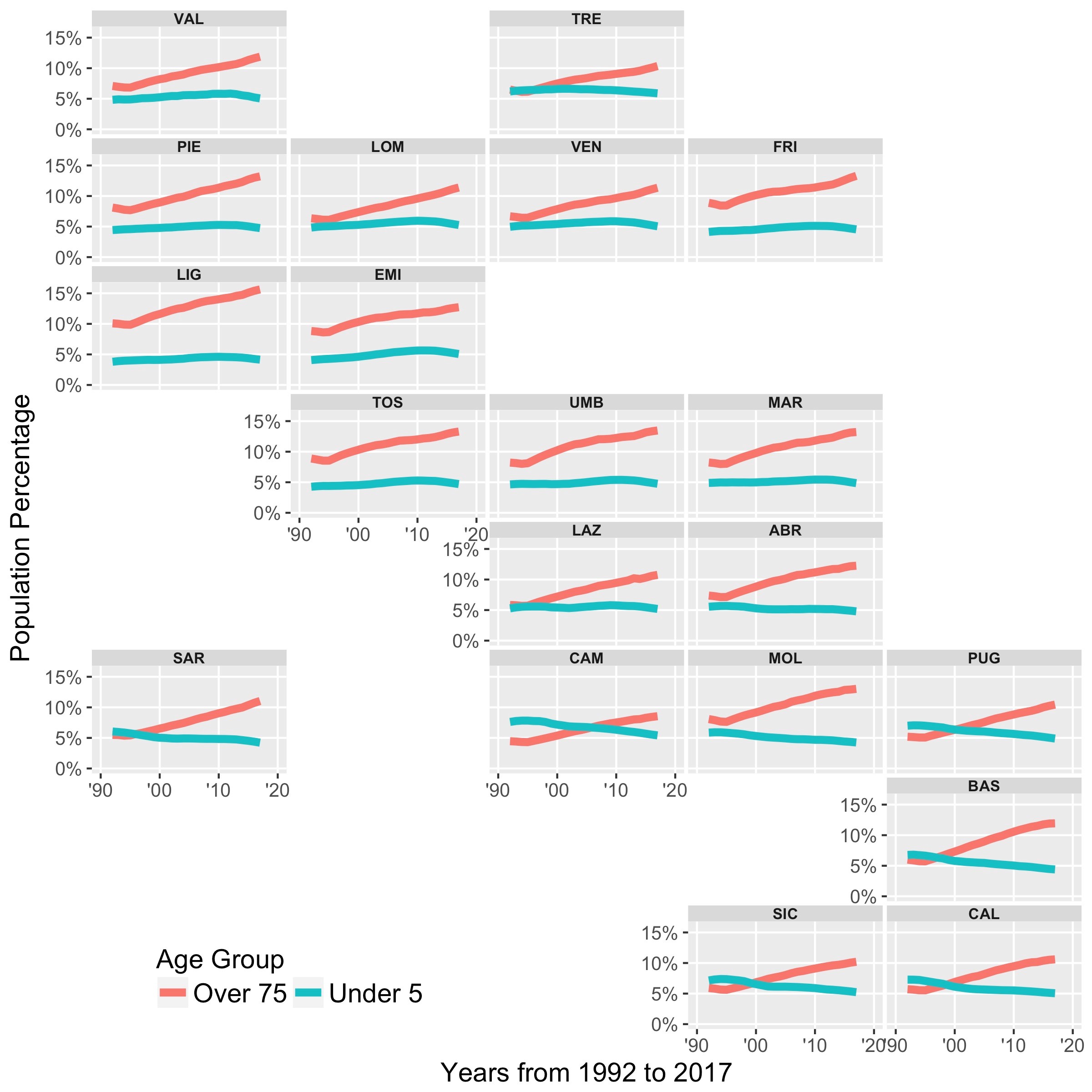
FIGURE 4 The percentage of the population aged under 5 years or over 75 years for the 20 Italian regions from 1992 to 2017.
The shape of Italy and the positioning of its regions make the construction of a grid for it difficult, and we acknowledge that variations on our grid that represent better the geographical layout are possible. Indeed, we have submitted two Italy grids to github. Hafen’s geofacet R package provides a simple-to-use contribution to the tool box of techniques for visualising spatial data that harnesses the power of ggplot2 in a reproducible way. The beauty of this approach is that people can improve on grids that have already been submitted and also contribute new grids for other countries, an activity that we strongly encourage.
Acknowledgements
We thank Daniela Antonelli, Mario Cortina Borja and Luisa Franconi for useful discussions.
About the authors
Stella Cangelosi is a student at Plymouth High School for Girls, Plymouth, who undertook work placement at Plymouth University. Luciana Dalla Valle is a lecturer in statistics in the School of Computing, Electronics and Mathematics, Plymouth University. Julian Stander is associate professor (reader) in mathematics and statistics in the School of Computing, Electronics and Mathematics, Plymouth University.
References
- Bivand, R. S., Pebesma, E. J. and Gómez-Rubio, V. (2008) Applied Spatial Data Analysis with R. Springer, New York. ^
- Wickham, H. (2016) ggplot2: Elegant Graphics for Data Analysis. Second Edition. Springer, New York. ^
- Lovelace, R., Cheshire, J., Oldroyd, R. and others. (2017) Introduction to Visualising Spatial Data in R. ^
- Cortina Borja, M., Stander, J. and Dalla Valle, L. (2016) The EU referendum: surname diversity and voting patterns. Significance, August 2016, Volume 13, Issue 4, pages 8-9. ^
- Wilkinson, L. (2005) The Grammar of Graphics. Second Edition. Statistics and Computing. Springer, New York. ^
- Hafen, R. (2017) geofacet: ggplot2 Faceting Utilities for Geographical Data. R package version 0.1.4. ^
- Kertzer, D. I., White, M. J., Bernardi, L. and Gabrielli, G. (2009) Italy’s path to very low fertility: the adequacy of economic and second demographic transition theories. European Journal of Population, 25, 89–115. ^
- https://www.istat.it/en/files/2017/07/Poverty-in-Italy_2016.pdf ^
- Vitali, A. and Billari, F. C. (2017) Changing determinants of low fertility and diffusion: a spatial analysis for Italy. Population, Space and Place, 23, 1–18. ^
- https://www.theguardian.com/world/2015/feb/13/italy-is-a-dying-country-says-minister-as-birth-rate-plummets ^


